HyperLogLog in Presto: Faster cardinality estimation

Computing the count of distinct elements in massive data sets is often necessary but computationally intensive. Say you need to determine the number of distinct people visiting Facebook in the past week using a single machine. Doing this with a traditional SQL query on a data set as massive as the ones we use at Facebook would take days and terabytes of memory. To speed up these queries, we implemented an algorithm called HyperLogLog (HLL) in Presto, a distributed SQL query engine. HLL works by providing an approximate count of distinct elements using a function called APPROX_DISTINCT. With HLL, we can perform the same calculation in 12 hours with less than 1 MB of memory. We have seen great improvements, with some queries being run within minutes, including those used to analyze thousands of A/B tests.

Today, we are sharing the data structure used to achieve these improvements in speed. We will walk through newly open-sourced functions with which we can further save on computations. Depending upon the problem at hand, we can achieve speed improvements of anywhere from 7x to 1,000x. The example use cases below show how to take advantage of these new functions.

What led to HyperLogLog?

Suppose you have a large data set of elements with duplicate entries chosen from a set of cardinality n and you want to find n, the number of distinct elements in the set. For example, you would like to compute the number of distinct people who visited Facebook in a given week, where every person logs in multiple times a day. This would result in a large data set with many duplicates. Obvious approaches, such as sorting the elements or simply maintaining the set of unique elements seen, are impractical because they are either too computationally intensive or demand too much memory. Let’s go through a journey of algorithms, in order of increasing complexity, to achieve our goal and fully understand how HLL works:

A simple estimator

To find our answer, we want an algorithm that outputs an estimate. That estimate may be in error, but it should be within a reasonable margin. First, we generate a hypothetical data set with repeated entries as such:

Generate n numbers evenly distributed between 0 and 1.
Randomly replicate some of the numbers an arbitrary number of times.
Shuffle the above data set in an arbitrary fashion.

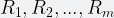
Since the entries are evenly distributed, we can find the minimum number ( $x_{min}$ ) in the set and estimate the number of unique entries as $1/x_{min}$ . However, to ensure that the entries are evenly distributed, we can use a hash function and estimate the cardinality from the hashed values instead of from the entries themselves. The graph below illustrates a simple example in which the hashed values are normalized and uniformly distributed between 0 and 1.

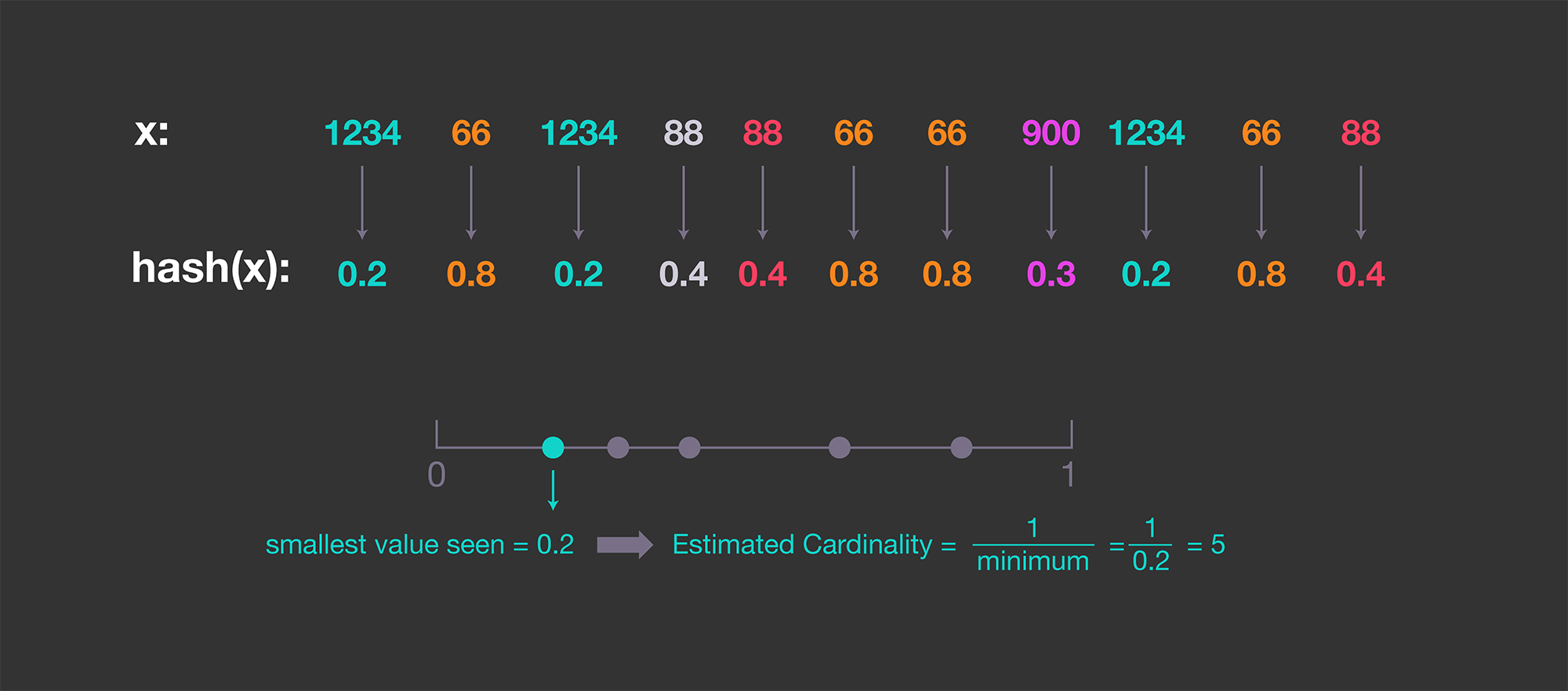
Although straightforward, this procedure has a high variance because it relies on the minimum hashed value, which may be happen to be too small, thus inflating our estimate.

Probabilistic counting

To reduce the high variability in previous method, we can use an improved pattern by counting the number of zero bits at the beginning of the hashed values. This pattern works because the probability that a given $hash(x)$ ends in at least i zeros is $1/2^i$ . The figure below illustrates an example of the probability of observing a sequence of three consecutive zeros.

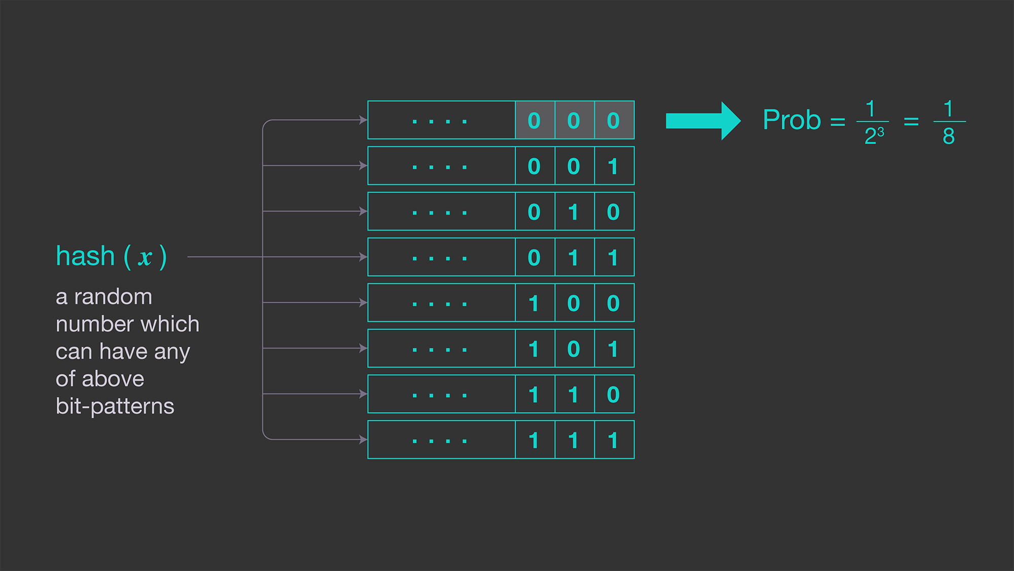
In other words, on average, a sequence of k consecutive zeros will occur once in every $2^k$ distinct entries. To estimate the number of distinct elements using this pattern, all we need to do is record the length of the longest sequence of consecutive zeros. Mathematically speaking, if we denote $\rho(x_i)$ as the number of consecutive zeros in $hash(x_i)$ , the cardinality of the set $\{x_1, x_2, ..., x_M\}$ is $2^R$ , where $R = \max\left(\rho(x_1), \rho(x_2), ..., \rho(x_M)\right)$ .

There are two disadvantages to this method:

At best, this can give us a power of two estimate for the cardinality and nothing in between. Because of $2^R$ in the above formula, the resulting cardinalities can only be one of $\{1, 2, 4, 8, 16, 32, ..., 1024, 2048, 4096, ...\}$ .
The estimator still has high variability. Because it’s recording the maximum $\rho(x_i)$ , it requires only one entry whose hash value has too many consecutive zeros to produce a drastically inaccurate (overestimated) estimate of cardinality.

On the plus side, the estimator has a very small memory footprint. We record only the maximum number of consecutive zeros seen. So to record a sequence of leading zeros up to 32 bits, the estimator needs only a 5-bit number for storage.

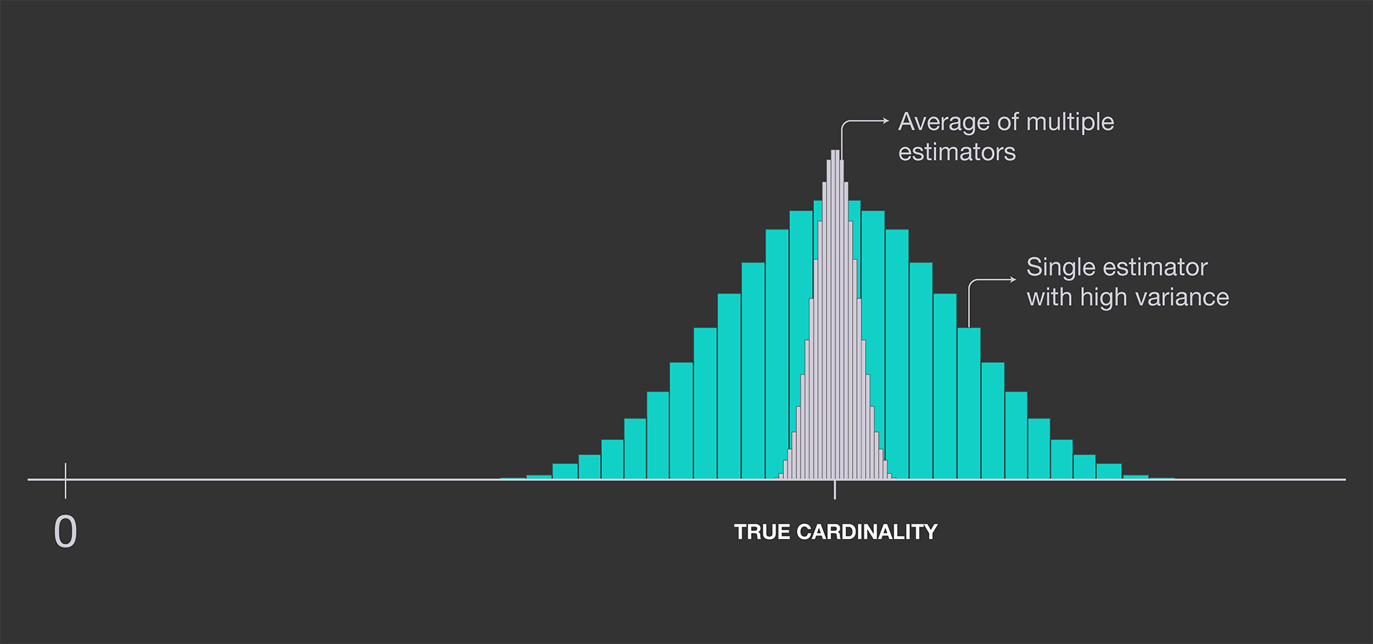
Improving accuracy: LogLog

In order to improve the estimate, we can store many estimators instead of one and average the results. This is illustrated in the graph below, where a single estimator’s variance is reduced by using multiple independent estimators and averaging out the results.

We can achieve this by using m independent hash functions: $\{h_1(x), h_2(x), ..., h_m(x)\}$ . Having obtained the corresponding maximum number of consecutive zeros for each one: ${R_1, R_2, ..., R_m}$ , our estimator becomes $2^{\bar{R}} = 2^{\frac{1}{m}\left(R_1+...+R_m\right)}$ .

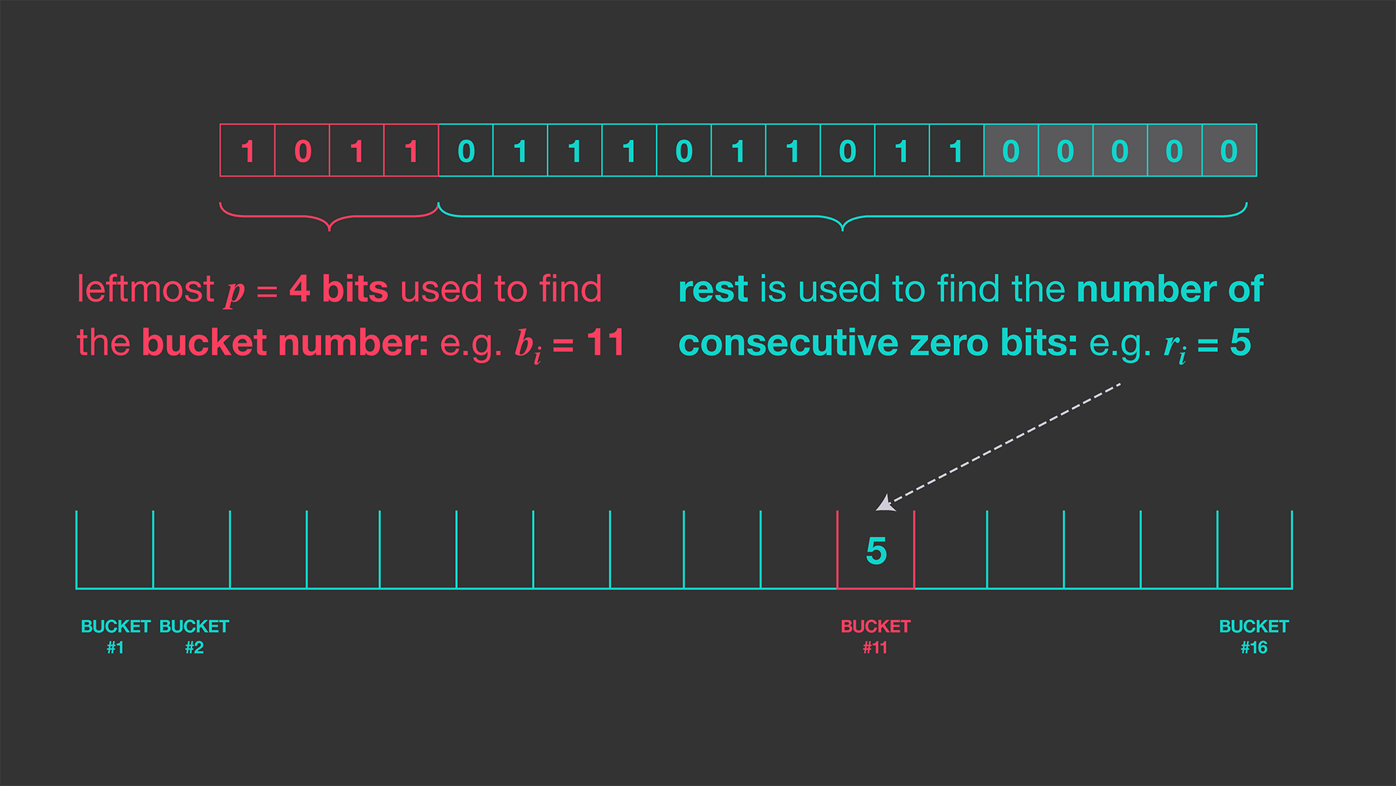
However, this requires each input $x_i$ to pass through a number of independent hash functions, which is computationally expensive. The workaround proposed by Durand and Flajolet is to use a single hash function but use part of its output to split values into one of many buckets. To break the input entry into m buckets, they suggest using the first few (k) bits of the hash value as an index into a bucket and compute the longest sequence of consecutive 0s on what is left (let’s denote the longest sequence as R).

For example, assume the hash of our incoming datum looks like hash(input)=1011011101101100000. Let’s use the four leftmost bits (k = 4) to find the bucket index. The 4-bits are colored: 1011011101101100000, which tells us which bucket to update (1011 = 11 in decimal). So that input should update the 11th bucket. From the remaining, 1011011101101100000, we can obtain the longest run of consecutive 0s from the rightmost bits, which in this case is five. Thus, we would update bucket number 11 with a value of 5 as illustrated below, using 16 buckets.

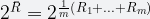
By having m buckets, we are basically simulating a situation in which we had m different hash functions. This costs us nothing in terms of accuracy but saves us from having to compute many independent hash functions. This procedure is called stochastic averaging. Finally, the formula below is used to get an estimate on the count of distinct values using the m bucket values $\{R_1, R_2,..., R_m\}$ .

$\text{CARDINALITY}_{\text{LogLog}} = \text{constant} \cdot m \cdot 2^{\frac{1}{m}\sum_{j=1}^N R_j}$

Statistical analysis has shown that the above estimator has a predictable bias towards larger estimates. Durand-Flajolet derived the constant=0.79402 to correct this bias (the algorithm is called LogLog).
For m buckets, this reduces the standard error of the estimator to about $1.3/\sqrt{m}$ . Thus, with 2,048 buckets where each bucket is 5 bits (which can record a maximum of 32 consecutive 0s), we can expect an average error of about 2.8 percent; 5 bits per bucket is enough to estimate cardinalities up to $2^{27}$ per the original paper and requires only 2048 * 5 = 1.2 KB of memory. That’s pretty good for basically 1 KB of memory.

HLL: Improving accuracy even further

Now that we’ve got a good estimator, we can do even better with two additional improvements:

Durand and Flajolet observed that outliers greatly decrease the accuracy of this estimator. Thus, the accuracy can be improved by throwing out the largest values before averaging. Specifically, when collecting the bucket values in order to produce the final estimate, accuracy can be improved from $1.3/\sqrt{m}$ to only $1.05/\sqrt{m}$ by only retaining the 70 percent smallest values and discarding the rest for averaging (this algorithm is called SuperLogLog).
HLL uses a different type of averaging in its evaluation function. Instead of the geometric mean used in LogLog, Flajolet et al. proposed using harmonic mean, edging down the error to slightly less than $1.04/\sqrt{m}$ with no increase in required storage.

Put all these pieces together and we get the HLL estimator for the count of distinct values.

$\text{CARDINALITY}_{\text{HLL}} = \text{constant} \cdot m \cdot \frac{m}{\sum_{j=1}^N 2^{-R_j}}$

Set operations on HLL

Set union operations are straightforward to compute in HLL and are lossless. To combine two HLL data structures, simply take the maximum corresponding bucket values of the two and assign that to the corresponding bucket in the unioned HLL. If we think about it, it is exactly as if we had fed in the union of the two data sets to one HLL to begin with. Such a simple set union operation allows us to easily parallelize operations among multiple machines independently using the same hash function and the same number of buckets.

Presto’s HLL implementation

Storage structure

The Presto-specific implementation of HLL data structures has one of two layout formats: sparse or dense. Storage starts off with a sparse layout to save on memory. If the input data structure goes over the prespecified memory limit for the sparse format, Presto automatically switches to the dense layout.

We introduced a sparse layout to ensure an almost exact count in low-cardinality data sets (e.g., number of distinct countries). But if the cardinality is high (e.g., number of distinct users), the dense layout will be what the HLL algorithm will produce as an approximate estimate. The handling of sparse to dense is taken care of automatically by Presto.

Sparse layout stores a set of 32-bit entries/buckets next to one another, sorted in ascending order by bucket index. As new data comes in, Presto checks whether the bucket number already exists. If it does, its value is updated. If the bucket is new, Presto allocates a new 32-bit memory address to hold the value. As more data flows in, the number of buckets may increase above a prespecified memory limit. At that point, Presto switches to a dense layout representation.

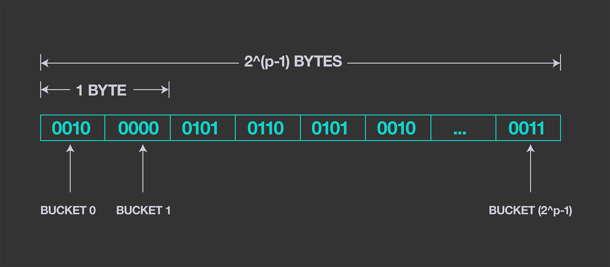
Dense layout has a fixed number of buckets and the associated memory is allocated from the beginning. Bucket values are stored as deltas from a baseline value, which is computed as: baseline = min(buckets). The bucket’s values are encoded as a sequence of 4-bit values, as shown in the figure below. Based on the statistical properties of the HLL algorithm, 4-bits is sufficient to encode the majority of the values in a given HLL structure. For deltas greater than $2^4$ , the remainders are stored in a list of overflow entries.

Data types

There is a HYPERLOGLOG data type in Presto. Since sparse and dense layouts have different performance and accuracy characteristics, some users may prefer a single format, such that they can process the output structure in other platforms (e.g., Python). Therefore, there is another data type, P4HYPERLOGLOG, which starts and stays strictly as a dense HLL.

P4HYPERLOGLOG implicitly casts to HYPERLOGLOG
HYPERLOGLOG can be explicitly casted to P4HYPERLOGLOG

Presto functions to work with HLL

These recently documented Presto functions allow users to exploit the HLL data structure with more detail and greater flexibility:

- APPROX_SET(x) -> HYPERLOGLOG
    This function will return the HLL sketch of the input set of data x.
- MERGE(hlls) -> HYPERLOGLOG
    This function does set union of a bunch of HLL sketches.
- CARDINALITY(hll) -> BIGINT
    This function will apply the HLL distinct count formula on the sketch and
    return the final number of distinct values.
- CAST(hll AS VARBINARY) -> VARBINARY
    In order to store the HLL sketch in Hive tables, we must CAST them to
    VARBINARY.
- CAST(varbinary AS HYPERLOGLOG) -> HYPERLOGLOG 
    In reading the stored HLL sketch from a table, we must CAST to HLL in order 
    to perform further merging and cardinality estimation.
- CAST(hll AS P4HYPERLOGLOG) -> P4HYPERLOGLOG 
    To enforce the dense layout of the HLL sketch, we can cast to P4HYPERLOGLOG.
- EMPTY_APPROX_SET() -> HYPERLOGLOG 
    This function returns an empty HLL sketch. It can be used in order to deal 
    with functions that should return the data of HYPERLOGLOG but instead return 
    NULL. For example, APPROX_SET(NULL) would return NULL instead 
    of an empty HYPERLOGLOG data structure, which could lead to other failures.

The following examples highlight the advantages of these functions:

Example 1: Applying COUNT DISTINCT at different levels of aggregation

Let’s assume we have a table with the following columns: job_id, server_id, cluster_id, datacenter_id, which incorporates information regarding the location in which a given job (e.g. Presto job) is running. In the above, a data center consists of multiple clusters, and each cluster has multiple servers.

A common use case with such a data set is answering the following:

Number of distinct jobs in each (server, cluster, data center)?
Number of distinct jobs in each (cluster, data center)?
Number of distinct jobs in each (datacenter)?

With a traditional approach, we would run a query using GROUPING_SETS and APPROX_DISTINCT:

SELECT
    datacenter_id,
    cluster_id,
    server_id,
    APPROX_DISTINCT(device_type) AS num_distinct_devices
FROM
    dim_all_info
GROUP BY GROUPING SETS (
    (datacenter_id),
    (datacenter_id, cluster_id),
    (datacenter_id, cluster_id, server_id));

The above approach (GROUPING SETS) requires multiple traversals of the data set for each grouping. At each traversal, Presto ends up recalculating APPROX_DISTINCT using HLL under the hood. We can reduce the overall computation by taking advantage of the HLL data structure associated with the most granular grouping of (server_id, cluster_id, datacenter_id); after which we can roll up the distinct counts for higher levels.
Imagine we have 1,000,000 rows consisting of 20 cluster_ids, each with 50 server_ids. We can apply APPROX_DISTINCT twice as follows:

APPROX_DISTINCT(x) ... GROUP BY (cluster_id, server_id) $\rightarrow 20 \times 50 = 1000$ rows
APPROX_DISTINCT(x) ... GROUP BY (cluster_id) $\rightarrow 20$ rows

We can sweep over the most granular level (cluster_id, server_id), but avoid the second full traversal by rolling up the results in the 1,000 rows associated with (cluster_id, server_id). From these 1,000 rows alone, you can actually get the distinct count BY cluster_id and obtain the same final 20 rows for each cluster.

Note: To illustrate how the Hive storage of this data structure can be implemented, we can create new tables in this process for each aggregation level, from most granular to least granular. However, their separate storage is not necessary (and can be held in memory) for the computation.

CREATE TABLE server_level_aggregates (
    datacenter_id VARCHAR,
    cluster_id VARCHAR,
    server_id VARCHAR,
    job_hll_sketch VARBINARY
)

INSERT INTO server_level_aggregates
SELECT
    datacenter_id, 
    cluster_id,
    server_id,
    CAST(APPROX_SET(job_id) AS VARBINARY) AS job_hll_sketch
FROM
    dim_all_jobs
GROUP BY
    1, 2, 3

Now that we have the table server_level_aggregates stored, if we want to know the count of distinct jobs per (server_id, cluster_id, datacenter_id) without resorting to the raw data set, we can simply do:

SELECT 
    datacenter_id,
    cluster_id,
    server_id,
    CARDINALITY(CAST(job_hll_sketch AS HYPERLOGLOG)) AS num_distincts
FROM 
    server_level_aggregates

The table server_level_aggregates has a much smaller number of rows than the original table dim_all_jobs. Having this table also allows us to roll up the number of distinct devices at the cluster or data center level. Since we have already stored the intermediate HLL data structure in table server_level_aggregates, lossless merging can be done when rolling up.

CREATE TABLE  cluster_level_aggregates (
    datacenter_id VARCHAR,
    cluster_id VARCHAR,
    job_hll_sketch VARBINARY 
)

INSERT INTO  cluster_level_aggregates
SELECT  
    datacenter_id, 
    cluster_id,
    CAST(
        MERGE(CAST(job_hll_sketch AS HYPERLOGLOG)) 
        AS VARBINARY 
    ) AS  job_hll_sketch
FROM 
    server_level_aggregates
GROUP BY 
    1, 2

Similarly, we can calculate the CARDINALITY for (cluster_id, datacenter_id) aggregates as follows:

SELECT  
    datacenter_id,
    cluster_id,
    CARDINALITY(CAST(job_hll_sketch AS HYPERLOGLOG)) AS num_distincts
FROM  
    cluster_level_aggregates

If we didn’t care about storing the HLL data structure in previous queries, we could have directly computed the cardinality:

SELECT 
    datacenter_id, 
    cluster_id,
    CARDINALITY(MERGE(CAST(job_hll_sketch AS HYPERLOGLOG))) AS num_distincts
FROM
    server_level_aggregates
GROUP BY
    1, 2

Example 2: Applying COUNT DISTINCT for any desired DS range

There are many instances in which we require the distinct count of grouped values for a varying range of dates. For example, we may have a weekly pipeline that calculates the COUNT(DISTINCT x) for 7, 28, and 84 days in the past. Or we may want to obtain COUNT(DISTINCT x) for any desired ds range for a data set which has strictly limited retention. HLL sketches allow for the calculation of the desired cardinality for any ds range while also saving on compute time.

If we had already calculated weekly partitioned HLL sketches in a table called weekly_hll_table, we could have merged four weekly partitions to obtain the cardinality for a month’s worth of data:

SELECT 
    CARDINALITY(MERGE(CAST(hll_sketch AS HYPERLOGLOG))) AS monthly_num_distinct
FROM
    weekly_hll_table
WHERE
    ds BETWEEN '2018-10-01' AND '2018-10-31'

If we have a pipeline that stores the daily HLL sketches in a table called daily_hll_table and we are interested in the cardinality of the data for some arbitrary time window in the past (e.g., the first half of July) we can achieve this without going over the original data set as follows:

SELECT 
    CARDINALITY(MERGE(CAST(hll_sketch AS HYPERLOGLOG))) AS num_distinct_mid_july
FROM
    daily_hll_table
WHERE
    ds BETWEEN '2018-07-01' AND '2018-07-15'

Approximation error

In an effort to evaluate the error rate as a function of the cardinality, we simulate 1,000 samples of random numbers across a range of cardinalities and evaluate the observed relative errors.

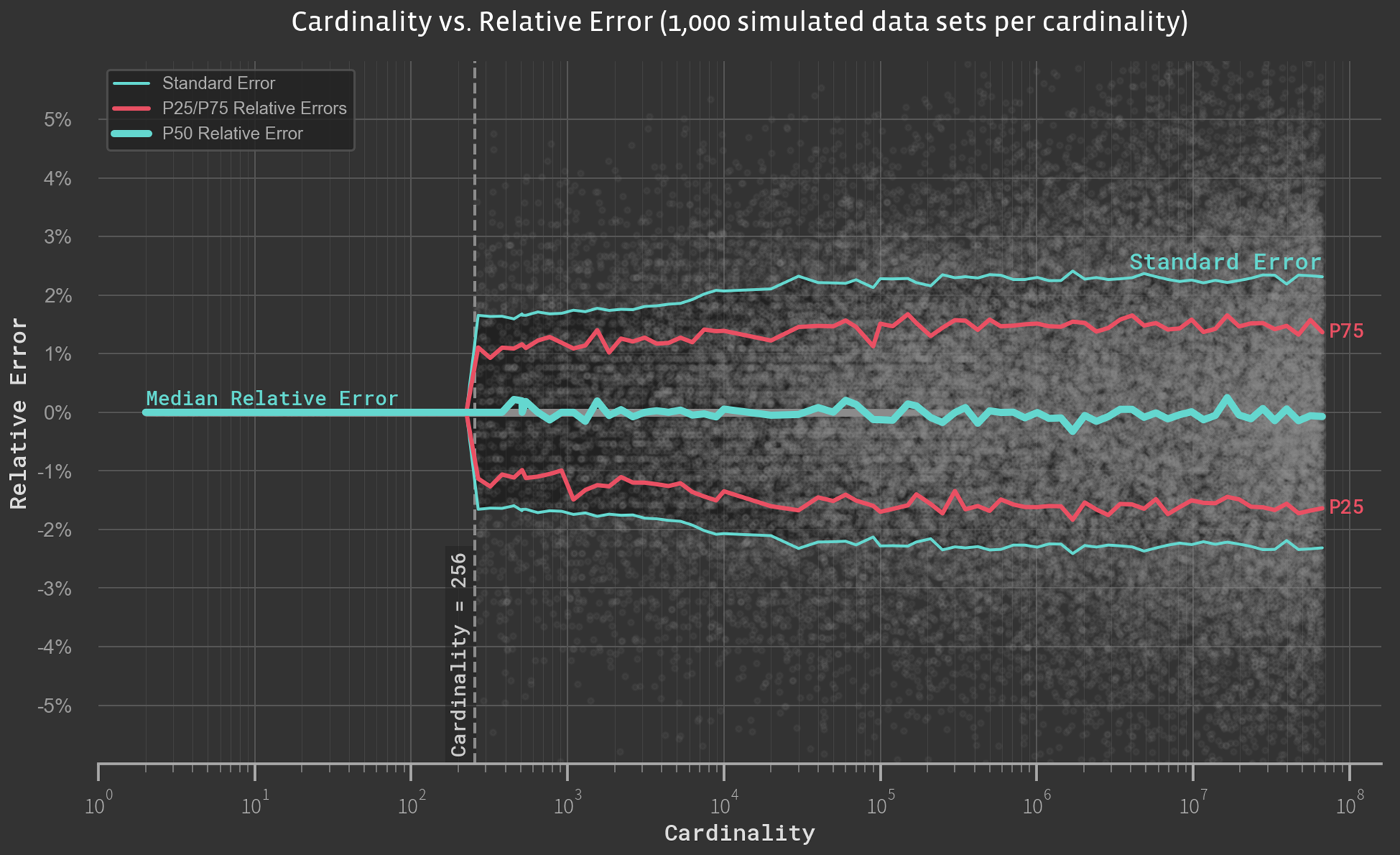
The standard error of the APPROX_DISTINCT function is observed as ~2.3 percent for all cardinalities above 256. For cardinalities below 256, the standard error is 0. This is because up to 256 unique elements APPROX_DISTINCT uses a sparse layout, which is an exact representation. For inputs with a larger number of unique elements, Presto switches to a ~8 Kb dense layout by default, resulting in an approximation error of 2.3 percent.

On the other hand, since APPROX_SET instantiates twice the number of buckets (4,096), the approximation error is reduced to 1.6 percent ( $1.04/\sqrt{4096}$ ). This can also be achieved by setting the optional parameter, e, in APPROX_DISTINCT(x, e), which represents the upper bound on the error.

What’s next?

HLL data structures can dramatically improve efficiency of cardinality estimations in terms of both the CPU cost and memory requirement. The HLL data structure requires approximately 1 KB of memory regardless of the input data set’s size. This has been useful in reducing the load on Facebook’s infrastructure, where queries and models run every day on massive amounts of data.

Presto now provides the functionality to access the raw HLL data structure that is used internally as part of APPROX_DISTINCT calculations. The functions described in this post allow users to write queries so as to reduce storage and computation costs, particularly in roll-up calculations. Further details on these functions can be found in the Presto documentation on HyperLogLog.

A parallel function for approximate percentile calculations (APPROX_PERCENTILE) has recently been incorporated into Presto as well. The data structure, called Q-Digest, is available as its own data type and offers the same advantages as APPROX_DISTINCT for percentile calculations. For more information, see Presto’s documentation on the Q-Digest data structure.