Whether it’s iterating on Facebook’s News Feed ranking algorithm or delivering the most relevant ads to users, we are constantly exploring new features to help improve our machine learning (ML) models. Every time we add new features, we create a challenging data engineering problem that requires us to think strategically about the choices we make. More complex features and sophisticated techniques require additional storage space. Even at a company the size of Facebook, capacity isn’t infinite. If left unchecked, accepting all features would quickly overwhelm our capacity and slow down our iteration speed, decreasing the efficiency of running the models.
To better understand the relationship between these features and the capacity of the infrastructure that needs to support them, we can frame the system as a linear programming problem. By doing this, we can maximize a model’s performance, probe the sensitivity of its performance to different infrastructure constraints, and study the relationships between different services. This work was done by data scientists embedded in our engineering team and demonstrates the value of analytics and data science in ML.
Supporting feature development
It’s important to continually introduce features that best leverage new data to maintain performant models. New features are responsible for the majority of incremental model improvements. These ML models are useful for our ad delivery system. They work together to predict a person’s likelihood of taking specific action on the ad. We work to continuously improve our models so our systems deliver only those ads that are relevant to a user.
As our techniques become more sophisticated, we develop more complex features that demand more of our infrastructure. A feature can leverage different services depending on its purpose. Some features have a higher memory cost, while others require extra CPU or take up more storage. It’s important to use our infrastructure wisely to maximize the performance of our models. We must be able to smartly allocate resources and be able to quantify the trade-offs of different scenarios.
To address these problems, we frame our system as a linear programming problem that maximizes our model’s metrics. We use this framework to better understand the interaction between our features and services. With this knowledge, we can automatically select the best features, identify infrastructure services to invest in, and maintain the health of both our models and services.
Framing our problem
To get a handle on our framework, we’ll first introduce a model problem. Say we have multiple features that all take up some amount of space (the height of the rectangles) and contribute some amount of gain to our models (the teal squares), and we are unable to accommodate them all in our limited capacity.
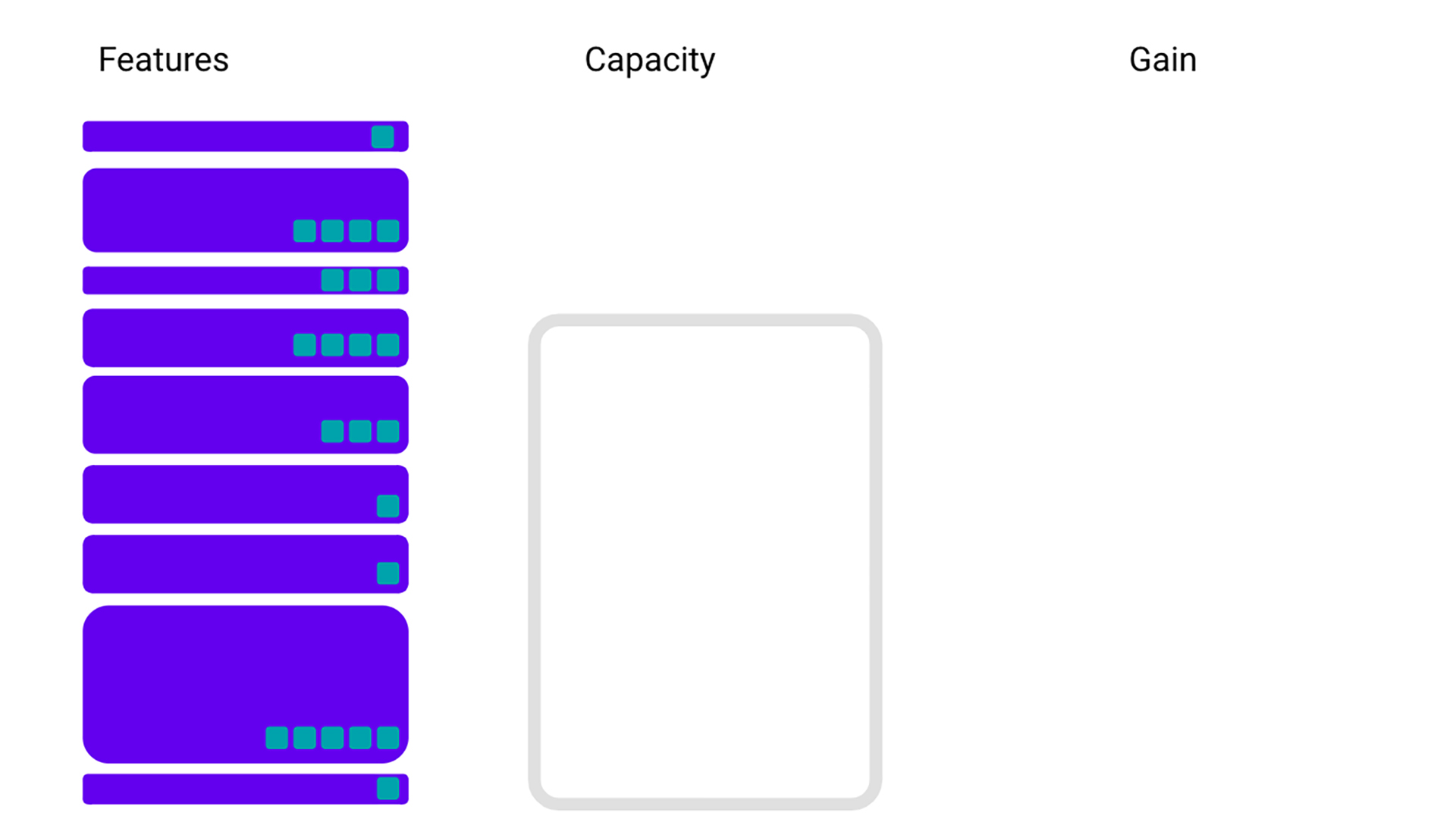
A naive solution would be to just start picking the features with the most gain (teal squares) until you are out of capacity. However, you might not be making the best use of your resources if you just prioritize the gain. For example, by taking in a big feature with a large gain, you could be taking up room that two smaller features with less gain could use instead. Together, those two smaller features would give you more bang for your buck than the big feature.
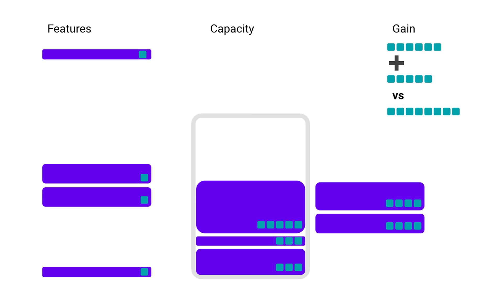
If we get a little less naive, we could instead look to pick features that give us the most bang per buck — features that have the most gain per storage. However, if we pick features only from that perspective, we could end up leaving out some less efficient features that we would still have room to accommodate.
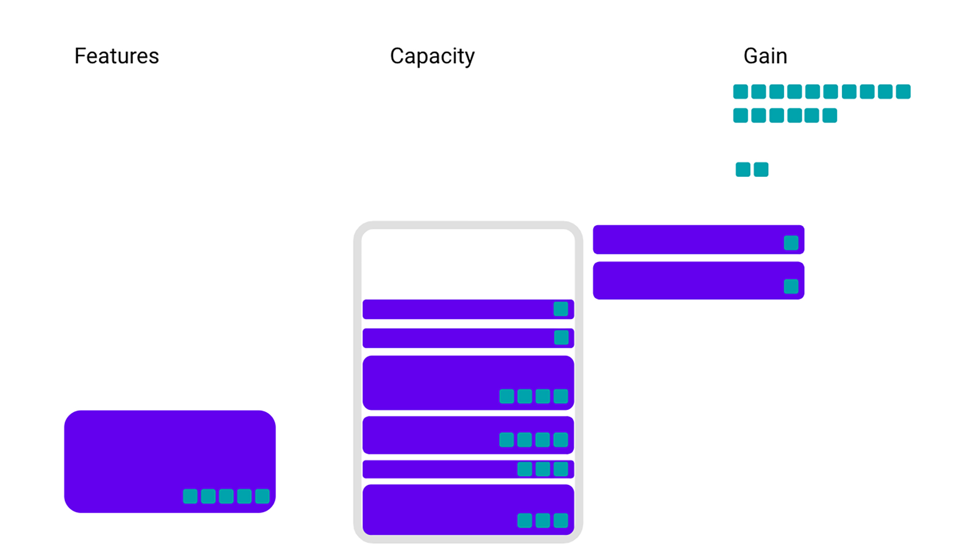
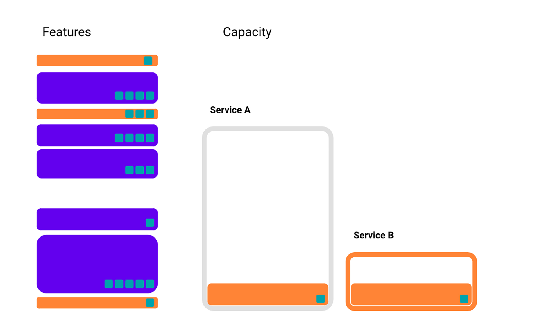
We’ve been looking at a very simplified view of infrastructure, but the reality is a bit more complex. For example, features often don’t take up just one resource but need many — such as memory, CPU, or storage in other services. We can make our example slightly more sophisticated by adding in Service B, and saying that orange features take up space in both Service A and Service B.
Picking which features we use is not the only way to control our infrastructure usage. We can also employ various techniques to increase the efficiency of our feature storage. This sometimes comes with a cost, either through the feature itself or capacity from a service. In this case, let’s say that we can halve the storage cost of some features (bordered in pink) but only at the cost of reducing the gain of the feature, and using some of the limited capacity in Service B.
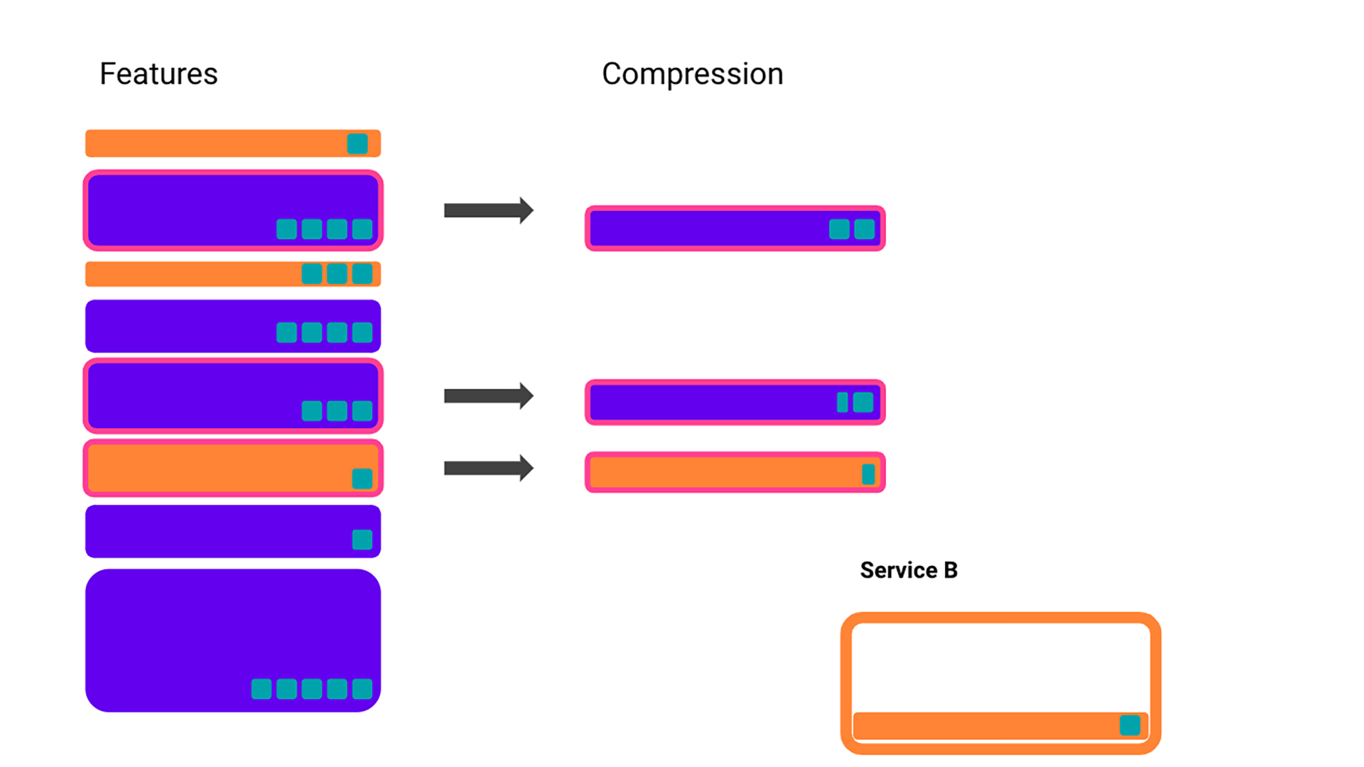
We’ll stop the example at this point, but this is enough for the general message to be clear — infrastructure can be a complicated interconnected system of different constraints. In reality, our capacity is not set in stone. We can move resources around if it is warranted. Features are also not the only thing we’re working on. There are plenty of other projects and workflows that compete for the same resources. We need to not only choose the features that maximize our gain but also be able to answer questions about how our system responds to changes:
- Which features do we select to optimize the gain?
- Is feature compression worth it? More important, is it worth an engineer’s time to implement it?
- How does the gain change if we add more capacity to Service A?
- How do service dependencies interact? If we increase the capacity of Service B, can we use less of Service A?
Scaling the problem
Let’s step back and review the conditions of our model problem:
- We want to maximize our gain.
- We are limited by the capacity of Service A.
- We are also limited by the capacity of Service B, which only some features contribute to.
- Some features may be compressed, but:
- They suffer a loss to their gain.
- Some of Service B’s capacity must be used.
We can express all these constraints as a system of linear equations.
Let 𝑥 be a vector that is 0 or 1 that signifies whether we select the feature, and let 𝑔 be a vector that stores the gain of the feature. The subscripts 𝑓 and 𝑐 denote whether we are specifying a full cost or compressed feature. For example, 𝑥𝑓 denotes full, uncompressed features that we have selected to include, and 𝑔𝑐 represents the cost of compressed features.
Given these definitions, our objective is to maximize:

We can now add our constraints that model the limitations of our infrastructure:
- Features will either be selected and compressed, selected but not compressed, or not selected. We should not select the compressed and uncompressed versions of the same feature.

- Let 𝑠 be the storage cost of the feature and the subscripts 𝐴 and 𝐵 represent Service A and B, respectively. For example, 𝑠𝐴𝑐 represents the storage cost of compressed features in Service A. We are constrained by the capacity of the two services.

- Some of Service B must be utilized to enable compression. Let’s represent that as a few features that must be selected.

With this, we have now completely specified our problem in a few equations and can solve them using linear programming techniques. Of course, as we are interested in automating and productionalizing this, it can easily be specified in code. For this example, we accomplish this in Python using the excellent NumPy and CVXPY packages.
import cvxpy as cp
import numpy as np
import pandas as pd

# Assuming data is a Pandas DataFrame that contains relevant feature data
data = pd.DataFrame(...)
# These variables contain the maximum capacity of various services
service_a = ...
service_b = ...

selected_full_features = cp.Variable(data.shape[0], boolean=True)
selected_compressed_features = cp.Variable(data.shape[0], boolean=True)

# Maximize the feature gain
feature_gain = (
   data.uncompressed_feature_gain.to_numpy() @ selected_full_features
   + data.compressed_feature_gain.to_numpy() @ selected_compressed_features
)

constraints = [
   # 1. We should not select the compressed and uncompressed version
   #    of the same feature
   selected_full_features + selected_compressed_features <= np.ones(data.shape[0]),
   # 2. Features are restricted by the maximum capacity of the services
   data.full_storage_cost.to_numpy() @ selected_full_features
   + data.compressed_storage_cost.to_numpy() @ selected_full_features
   <= service_a,
   data.full_memory_cost.to_numpy() @ selected_full_features
   + data.compressed_memory_cost.to_numpy() @ selected_compressed_features
   <= service_b,
   # 3. Some features must be selected to enable compression
   selected_full_features >= data.special_features.to_numpy(),
]
Leveraging the framework
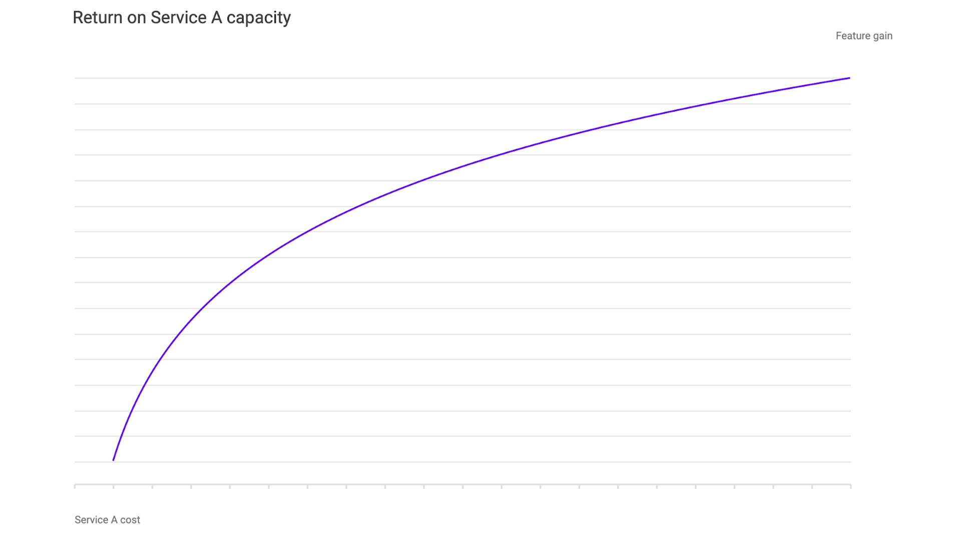
Now we have a framework that we can use to express our questions and hypotheticals. If we want to find out how an increase in Service A translates to a feature gain, we can run the optimization problem above at different values for Service A capacity and plot the gain. This way, we can directly quantify the return for each incremental increase in capacity. We can use this as a strong signal for what services we should invest in for the future and directly compare the return on investment on more feature memory, computing, or storage.
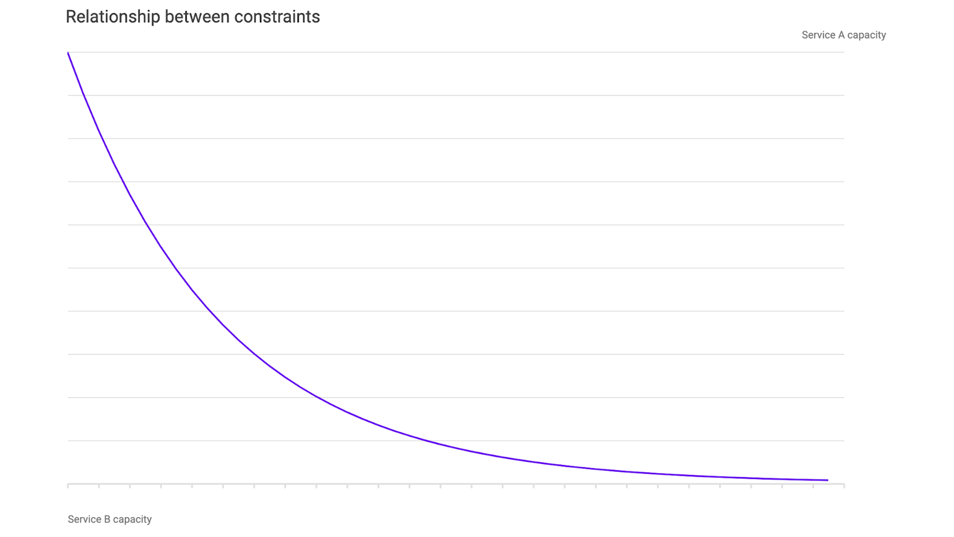
Similarly, we can look at the relationships between services. We simply vary the capacity of Services A and B while keeping the gain constant. We can see that as Service B’s capacity increases, less of Service A is needed to achieve the same gain. This can be leveraged if one service is overly stressed compared with another.
Linear programming as a framework for automating decisions
Previously, feature approval was a manual process where teams would spend valuable time calculating how many features we could support and analyzing what the return on investment was for increasing the capacity of our services. In a company like Facebook — where we have multiple models being continuously iterated on — this approach does not scale. By framing our services as a system of linear equations, we take a complex interconnected system and simplify it into basic relationships that are easily communicated. By doing this, we can make smarter decisions about the features we deploy and the infrastructure we invest in.


